Vector Signal Analyzers (VSAs) are powerful instruments that allow you to examine your signals in multiple domains simultaneously. They combine the traditional spectrum analyzer functionality in the frequency domain with powerful time domain capability. This not only gives you the ability to observe spectral changes over time, but also the ability to examine other characteristics vs. time. This includes basic parameters such as amplitude, frequency and phase deviation vs. time, as well as more complex measurement functions such as analog and digital modulation analysis, radar and pulsed RF analysis.
Traditional spectrum analyzer users find that the frequency domain controls (center frequency, span, RBW) are all very familiar on a VSA. However, adding the additional dimension of time also adds another layer of controls needed to setup the time-domain aspects of the instrument. In the past, managing the combination of frequency domain and time domain controls in a VSA could be confusing. Modern instruments, like the Tektronix RSA series of spectrum analyzers, incorporate features in the user interface to make managing these domains clear and intuitive.
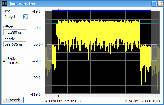
The user interface in these instruments includes a display called the “Time Overview.” This graphical display gives you the ability to visually observe and control the length or duration of the seamless acquisition of data, and control which portion of an acquisition you wish to analyze in the time domain and frequency domain. The controls and display features in this window make it easy to “see” what the instrument is analyzing and make adjustments as needed.

The Time Overview display shown above shows a time-domain plot of the acquired signal’s amplitude vs. time. Note that this is the total amplitude within the bandwidth used for the acquisition. In this case, a ~560 µs burst of a modulated RF signal is shown. The trigger position is indicated by the red T along the bottom of the graphic window.
The blue bar along the top of the graphic window indicates the Analysis Region. It is this portion of the acquisition that the time domain analysis displays will be computed. These include any display that includes a time axis (Amplitude / Frequency / Phase / IQ vs time, spectrogram), as well as any of the modulation analysis or pulse analysis, displays. When “Analysis” is selected in the Time: dropdown box in the upper left corner of the display, the Analysis Region is indicated by the shadow curtains on waveform graphic area.

There are two controls for the Analysis Region – the Analysis Offset and the Analysis Length. These are controlled using the numeric Offset: and Length: fields on the left edge of the display. The offset is the starting position of Analysis Region – i.e. the left edge of the blue bar. The Analysis Length, or the length of the blue bar, is controlled by the second button. The analysis length shown is 683.636 µs. The analysis offset shown is ‑42.388 µs. The negative number indicates that the start of the analysis region is before the trigger event (pre-trigger).

The Analysis Region controls which portion of the acquisition is analyzed in nearly all of the other displays, with the notable exception of the Spectrum Display.
The Spectrum Display result is computed from the acquisition in the area indicated by the Spectrum Region – the red bar on the Time Overview display. By selecting “Spectrum” from the Time: dropdown box in the upper left corner of the display, the Spectrum Time is indicated by the shadow curtains in the graphic. The numeric values for the offset and length can be entered by clicking each numeric field and entering the value, or by clicking and dragging the edges of the shadow under the red bar.

You can manually adjust the Spectrum Length, but you should be aware of how this will affect the resulting Spectrum Display. If you manually adjust the Spectrum Length to a value that is shorter than the auto-set value, then the RBW in the Spectrum Display will increase. There will be an indication of this in the lower left corner of the spectrum display that will indicate “RBW increased to xxx”.
If you manually adjust the Spectrum Length to a value that is longer than the auto-set value, it will potentially cause multiple spectrum calculations to be performed. Here’s how it works…
- If the Spectrum Length is increased by less than 2x, there is no change in how the spectrum is computed.
- If the Spectrum Length is increased by 2x or more, then multiple individual spectrum results are computed from adjacent locations in time. The first spectrum calculation is done starting at the spectrum offset. The next is calculated immediately adjacent to the first spectrum calculation. This process continues for as many integer multiples of the (auto-set) spectrum lengths as will fit within the user set spectrum length. Then, each of these resulting spectrum calculations are passed through the Trace Detector that is selected in the Spectrum Trace settings.
- In all cases, the RBW used is the RBW setting requested in the spectrum display.
For example, if the spectrum length was increased by a factor of 5, then 5 spectrum results are calculated successively through the time period indicated by the red bar. Each of those results are passed through the trace detector. If the detector was set to “average”, then the result will be the average of the 5 calculations. If it was set to +Peak, then the resulting trace will be the composed of the highest amplitude of all the results at each frequency.
The pink bar at the bottom of the graphic display is a “results” indicator. As you select the various displays that you have open, the pink bar at the bottom of the Time Overview display will graphically show you the region where those results were calculated. This is very helpful when you are moving the Analysis Region around, or you are performing measurements such as a constellation diagram, where there is no time axis. It also makes it clear when you need to “replay” the data to refresh your measurement across a newly defined analysis region.

The Tektronix family of Spectrum Analyzers includes the Time Overview display to make it easy to control how much time you wish to acquire, and what portions of that acquisition you want to analyze in the different domains. This same user interface is also used in Tektronix Vector Signal Analysis software, called SignalVu and SignalVu-PC. SignalVu is an option available most of the current windows-based oscilloscopes ranging from 500MHz to 70GHz bandwidth. SignalVu-PC is a standalone PC application which is used to control any of the USB-based RSAs (RSA300/500/600 series), and can also be used to perform offline vector signal analysis on data collected on any of the RSAs, oscilloscopes, as well as data from MATLAB.